This post is my build log for the Leaky Integrate-and-Fire neuron, usually called the LIF model. What I created was my own implementation of it, starting from the book, then extending it with firing-rate curves, refractory periods, and a few biological interpretations.
The surprising part is that the model is extremely simple. A neuron is treated like a tiny electrical circuit: the membrane stores charge like a capacitor, current pushes the membrane voltage upward, and leak channels pull it back toward a resting value. When the voltage crosses a threshold, I record a spike and reset the voltage.
That is enough to create a first computational model of a spiking neuron.
The core idea: integrate, leak, then fire
The LIF model tracks one main variable: the membrane potential, which I write as V. This is the voltage difference between the inside and outside of the neuron.
The equation I used is:
where:
Symbol | Meaning |
|---|---|
membrane capacitance, how much charge the membrane can store | |
leak conductance, how easily charge leaks out | |
leak reversal potential, the voltage the cell relaxes toward | |
injected current | |
membrane potential |
The equation has two parts.
First, the input current pushes the voltage up. Second, the leak term pulls the voltage back toward . This is why the model is called leaky integrate-and-fire. It integrates incoming current, but the integration is imperfect because charge leaks away.
In code, I wrote that continuous equation as one explicit Euler update:
dV = (I(i) + G_L*(E_L - V(i-1))) / Cm;
V(i) = V(i-1) + dt*dV;
Then I add the firing rule:
The spike/reset part is the discrete event rule layered on top of the voltage update:
if V(i) >= Vth
    spikes(i) = true;
    V(i-1) = Vpeak;
    V(i) = Vreset;
end
In my simulation, I used values similar to the tutorial code:
Parameter | Value used |
|---|---|
Leak potential, | -70 mV |
Threshold, | -50 mV |
Reset, | -65 mV |
Potassium reversal, | -80 mV |
Membrane capacitance, | 100 pF |
Membrane resistance, | 100 MΩ |
Leak conductance, | 10 nS |
Charge, leak, cross a threshold, reset
Exact constant-current LIF modelChange current, threshold and time constant to see the exact voltage trace and spike count.
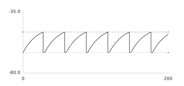
Interactive controls load when this figure enters view.
The leaky integrate-and-fire model uses a fixed rest voltage of −65 mV, resistance of 10 MΩ and 2 ms refractory period. Constant-current segments are integrated analytically over 200 ms. The vertical drops mark threshold/reset events, not biological action-potential waveforms or measured neurons.
My first simulation
I simulated the neuron under three injected currents: 180 pA, 220 pA, and 500 pA.
The sweep itself just loops over input currents and stores the two summaries I cared about:
for k = 1:numel(currents)
    I = currents(k) * ones(size(t));
    [V, spikes] = simulate_lif(I, params);

    meanV(k) = mean(V);
    rate(k) = sum(spikes) / tmax;
end
At 180 pA, the voltage rises but never crosses the threshold. The neuron stays silent.
At 220 pA, the voltage crosses threshold, spikes, resets, and repeats. This is the first point where the model behaves like a spiking neuron.
At 500 pA, the voltage reaches threshold much faster after every reset, so the neuron fires at a higher rate.
One important detail: when I plot the voltage trace, the tall spike line is not generated by the LIF differential equation itself. In the basic LIF model, the spike is added as a plotting convention. The actual rule is just: cross threshold, record spike time, reset voltage. This is a simplification compared with real neurons, where sodium and potassium channels create the full action potential shape.
Threshold current: when does the neuron start firing?
The steady-state voltage is the value the neuron would approach if I ignored the spike-and-reset rule:
The neuron starts firing only if this steady-state value is above threshold. So the threshold current is:
Using my parameters:
That matches the simulation: 180 pA is below threshold, 220 pA is above threshold.
The firing-rate curve: input current becomes spike rate
After getting spikes, I wanted to know how the firing rate changes as I increase injected current. This is called the f-I curve, firing rate versus input current.
The key observation is simple: more current means the voltage reaches threshold faster, so the neuron fires more frequently.
For the LIF model, the firing rate can be calculated analytically. The interspike interval is:
and the firing rate is:
where:
The curve is sharp near threshold because the ideal LIF model is deterministic. Below threshold, no spikes. Just above threshold, spikes suddenly appear. If I add noise to the voltage update, the threshold becomes softer because random fluctuations can occasionally push the membrane above threshold even when the average input is slightly too small.
What is the Nernst potential?
While building the refractory version of the model, I had to understand reversal potentials, especially the potassium reversal potential .
The Nernst potential is the voltage at which one ion species has no net driving force across the membrane. For an ion like potassium, it depends on the ratio of outside concentration to inside concentration:
Here, and are the outside and inside ion concentrations. In plain English: if potassium concentration changes outside the cell, the voltage that balances potassium movement also changes.
This matters because the resting membrane potential is strongly influenced by potassium leak channels. If extracellular potassium is reduced, the outside-to-inside potassium concentration ratio becomes smaller, so becomes more negative. Since resting voltage is pulled toward potassium's reversal potential, the neuron becomes more hyperpolarized, meaning its resting membrane potential moves farther from threshold.
In the tutorial code, I used mV for the refractory conductance model. When a potassium-like refractory conductance opens after a spike, it pulls the voltage downward toward , which helps prevent immediate re-spiking.
Adding a refractory period
Real neurons cannot fire again immediately after a spike. This short recovery window is called the refractory period.
I implemented three versions of a refractory LIF neuron.
I kept the refractory variants behind one method switch so the comparison stayed clean:
switch method
    case "clamp"
        inRefractory = t(i) < lastSpike + tRef;

    case "threshold"
        Vth(i) = Vth(i-1) + (Vth0 - Vth(i-1))*dt/tauVth;

    case "conductance"
        Gref(i) = Gref(i-1) * (1 - dt/tauGref);
        Iref = Gref(i) * (EK - V(i-1));
end
Method | What I changed | Biological idea | Line style in my plots |
|---|---|---|---|
Forced voltage clamp | Hold voltage at reset after a spike | Simple absolute refractory period | blue solid line |
Raised threshold | Increase threshold after a spike, then let it decay | Harder to spike immediately after firing | orange dotted line |
Refractory conductance + raised threshold | Add a temporary potassium-like conductance and raise threshold | More biophysical than a hard clamp | yellow dashed line |
The next six figures are for the refractory extensions, not the first basic LIF simulation. I arranged them in this order: first the summary behavior, then the voltage traces that explain why the curves look different.
Mean voltage as input current increases
Figure 1 shows the mean membrane potential as applied current increases. This is useful because two models can produce spikes but still have different voltage behavior between spikes. The forced voltage clamp can push the mean voltage downward at high input because the neuron spends more time artificially held at reset. The raised-threshold method behaves more naturally because the voltage is allowed to keep evolving after reset.
Firing-rate curve
Figure 2 shows the firing rate as a function of applied current. This is the main f-I curve for the refractory models. The raised-threshold model fires fastest because the membrane voltage is not clamped down after each spike. The forced-clamp model is slower because the neuron must wait through a fixed refractory window. The refractory conductance model is also slower because the temporary potassium-like conductance pulls the voltage downward after each spike.
Mean voltage versus firing rate
Figure 3 compares mean membrane potential directly against firing rate. This makes the modeling tradeoff clearer. A simple refractory clamp is computationally easy, but it can distort the voltage statistics. A dynamic threshold or conductance-based refractory mechanism preserves more of the voltage dynamics.
Forced voltage clamp trace
Figure 4 shows the forced voltage clamp method. After each spike, the membrane potential is held at the reset value for the refractory period. This is the simplest implementation, but it is also the most artificial because the voltage is manually fixed instead of being shaped by an ionic current.
Raised-threshold trace
Figure 5 shows the raised-threshold method. The voltage resets after a spike, but the threshold temporarily increases and then decays back. This separates the idea of resetting voltage from the idea of preventing another spike.
Refractory conductance with raised threshold trace
Figure 6 shows the refractory conductance method combined with a raised threshold. Here, the voltage drops more biologically because the refractory conductance acts like a temporary potassium current. Instead of manually forcing the voltage to stay low, the model creates a current that naturally pulls the membrane potential downward toward the potassium reversal potential.
The main lesson is that different simplifications can give similar spike trains but different voltage statistics. If I only care about spike times, a hard reset might be enough. If I care about the mean voltage, refractory conductance or dynamic threshold is more realistic.
Spike-rate adaptation
The next extension is spike-rate adaptation. In many real neurons, the first few spikes after a current step are close together, but later spikes spread farther apart.
This can be modeled by adding a slow potassium-like conductance that increases after each spike and decays slowly between spikes. It is similar to the refractory conductance idea, but with two key differences:
Adaptation uses the same state-variable pattern, just with a slower decay and a smaller jump:
Gadapt(i) = Gadapt(i-1) * (1 - dt/tauAdapt);

if spikes(i)
    Gadapt(i) = Gadapt(i) + deltaGadapt;
end
Feature | Refractory conductance | Adaptation conductance |
|---|---|---|
Strength | large | smaller |
Timescale | fast, a few ms | slow, often hundreds of ms |
Effect | prevents immediate next spike | gradually slows firing |
Purpose | enforces recovery | encodes recent spiking history |
So refractory period and spike-rate adaptation are similar computationally: both can use a conductance that jumps after spikes and decays over time. But biologically and dynamically, they are different. Refractory conductance prevents immediate firing. Adaptation conductance changes the firing pattern over a longer window.
Could adaptation make a neuron fire a few times and then stop forever?
In the simple adaptation model I implemented, the answer is no, not if the applied current remains truly above threshold.
And the reason, the adaptation conductance only increases when spikes happen. If the neuron stops spiking, the adaptation conductance decays back toward zero. Once it decays enough, the same applied current can push the voltage back to threshold again. So adaptation can slow firing or create a long pause, but it cannot permanently silence a suprathreshold LIF neuron by itself.
The only exception would be if the model included some nonzero adaptation current that persists without spikes, or if the applied current was actually below threshold and the early spikes were caused by a transient or noise.
Chapter question checks I worked through
After building the model, I also used it to sanity-check a few chapter-style questions. I treat this section as a short appendix rather than a new model.
1. What happens if extracellular potassium is reduced?
The resting membrane potential becomes more negative. Reducing extracellular potassium makes the potassium Nernst potential more negative, and since resting voltage is strongly influenced by potassium conductance, the neuron hyperpolarizes.
2. Steady-state voltage and firing rate calculation
This calculation uses a separate chapter parameter set from the earlier simulation. Using the common interpretation of those parameters:
For 6 nA:
So the steady-state membrane potential would be -10 mV if the reset rule were ignored. In the actual LIF model, the neuron would spike before sitting at that voltage.
For 15 nA:
The membrane time constant is:
Then:
So the firing rate is:
This is the no-refractory firing rate. If I added a refractory period, the rate would be lower.
3. Two similarities and two differences between refractory period and adaptation conductance
Similarities:
Both are usually triggered by spikes.
Both can be modeled with an extra state variable that decays over time.
Differences:
Refractory mechanisms are short and strong. Adaptation is slower and weaker.
Refractory mechanisms prevent immediate spiking. Adaptation mainly reduces the firing rate over time.
4. Can simple adaptation cause a few spikes and then permanent silence?
Not in the basic spike-triggered adaptation model. If spikes stop, the adaptation conductance decays. If the input current is still above threshold, the neuron should eventually spike again.
What the LIF model gets right and wrong
The LIF model gets the basic input-output logic right. It captures how injected current can push membrane voltage toward threshold and how stronger current produces higher firing rates.
But it is not a full biological neuron.
It does not model voltage-gated sodium channels, voltage-gated potassium channels, calcium dynamics, dendrites, ion-channel modulation, or spatial structure. It also uses an artificial threshold and reset rule instead of generating a real action potential.
That is why models like ELIF and AELIF exist.
The Exponential LIF model adds an exponential term near threshold, which makes the voltage accelerate upward like a real spike onset. The Adaptive Exponential LIF model adds adaptation, allowing richer firing patterns. But if the goal is to understand ion-channel mechanisms directly, then eventually we need conductance-based models such as Hodgkin-Huxley.
What I learned
Building this model made the theory feel concrete.
The LIF neuron is not powerful because it is biologically complete. It is powerful because it gives a clean bridge between electrical intuition and computational neuroscience. It teaches how voltage integrates input, how leak creates a timescale, how threshold creates spikes, how firing rate emerges from current, and how small modeling choices can change the interpretation of neural behavior.